One of the most commonly used SMLM techniques to visualize molecules and protein-protein interactions is direct STochastic Optical Reconstruction Microscopy (dSTORM). dSTORM is a complex method that requires researchers to pay particular attention during sample preparation, image acquisition, and computer analysis. Here we share some tips to help you improve your dSTORM imaging by tweaking your sample preparation, image acquisition and data analysis.
Sample preparation
Although often overlooked, sample preparation is key to achieve an optimal signal-to-noise ratio, which will result in a good quality super-resolution image. There are multiple protocols available for immunofluorescence staining for both conventional fluorescent (confocal, widefield, etc.) and super-resolution microscopy. In general, sample preparation for dSTORM imaging consists of three main steps: fixation and blocking, probing or labeling of your protein of interest, and signal enhancement.
Fixation and Blocking
The type of fixative used to fix your biological sample will depend on your protein of interest. Some fixatives can alter the epitope recognized by the primary antibody and thus will affect probing with primary antibodies. There are different fixatives that are used to fix biological samples, such as paraformaldehyde (PFA), methanol, glutaraldehyde or a combination of these. The most common fixation method is 4% PFA in phosphate buffer saline (PBS). The mechanism of fixation is dependent on the reagent used. For PFA, fixation starts immediately and 20 minutes is usually sufficient time to properly cross-link all proteins. After fixation and washing, the next step is blocking. Blocking is a very important step in sample preparation because it prevents the nonspecific binding of antibodies or other reagents to your sample. Which blocking reagent to use will depend on your target but for surface proteins blocking with 5% bovine serum albumin (BSA) in PBS is commonly used. However, if your aim is to stain intracellular proteins, you need to perform a permeabilization step as well. This can be done by incubating the sample with 0.1% Triton X-100 in PBS for at least 10 minutes prior to the blocking step, for example, or you can perform both blocking and permeabilization steps together by incubating the sample with 5% BSA with 0.1% Triton X-100 in PBS. Usually samples are blocked for 60 minutes at room temperature but can be blocked for longer, for example, overnight at 4℃. Importantly, insufficient blocking can lead to high nonspecific background levels and poor dSTORM image. We recommend using 5% BSA in PBS for 60 min as a starting point for blocking, and further optimize from there.
Probing
After blocking, the sample is now ready for probing. The most common way to stain molecules of interest is with primary antibodies. These can be unconjugated or conjugated to dSTORM-compatible fluorophores, for more information check our list of fluorophores compatible with STORM imaging. Staining is performed in the same buffer as the blocking step. If you are staining for intracellular proteins you can use the blocking/permeabilization buffer (5% BSA with 0.1% Triton X-100). This step will usually take another 60 minutes to complete at room temperature; alternatively you can stain with primary antibodies overnight at 4℃. If using primary antibodies directly conjugated to dSTORM-compatible dyes, the sample is ready for imaging after a washing step.
When considering how to label your structure of interest for dSTORM imaging, it is important to know the expression level of the target protein(s). If your target protein is highly expressed (e.g. 𝛼/β-tubulin) you will need to use a higher concentration of antibody (maximum 20 µg/mL) to ensure you label each individual protein in comparison to a protein that is not so highly expressed. In the latter case a lower concentration of antibody (1 µg/mL) could be enough to fully label each individual protein of interest. Ensuring your target protein is fully labeled is crucial for dSTORM imaging, you can do this by performing a titration of the antibody.
Under-labeled samples may still produce a good enough signal-to-noise ratio for conventional diffraction-limited microscopy techniques such as confocal or widefield microscopy. However, for dSTORM imaging, an underlabeled sample will not allow the visualization of the full structure with subnanometer resolution. We present an example of this, with the nuclear pore protein Nup98 (Figure 1). Labeling Nup98 with either 1 or 5 µg/mL of antibody does not make a difference in diffraction-limited imaging, however, differences will be observed in your dSTORM imaging. In a super-resolved image of nuclear pores, we would expect to see from five to six subunits of the nuclear pore ring, but as seen in the zoomed images below (Figure), we can only count two to three subunits when the sample is stained with 1 µg/mL of Nup98 antibody. On the other hand, when using 5 µg/mL of Nup98 antibody each subunit of the nuclear pore is resolved and the rendered image closer represents the full biological structure (Figure 1). This example highlights the importance of labeling density for dSTORM imaging. If your protein of interest is not well labeled with an antibody at a concentration of 20 µg/mL, most probably the antibody is not suitable for immunofluorescence. In this case, we advise you to test different clones of antibodies.
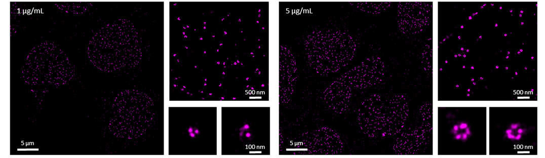
Figure 1. dSTORM images of the nuclear pore subunit protein Nup98 in primary T cells. Cells were probed with 1 or 5 µg/mL of primary antibody against Nup98 directly conjugated to AlexaFluor647.
Here are our two main tips for optimizing the labeling density of your target of interest:
- Perform a titration of the primary antibody to achieve the best labeling density for low- or high-expression targets. Use 5 µg/mL of primary antibody as a starting point.
- As a rule of thumb, for STORM imaging, you should likely be using at least twice the concentration of antibody that you use in conventional immunofluorescence microscopy (confocal or widefield).
Probing
The number of fluorophores per antibody can be a limiting factor to obtain a good quality super-resolution dSTORM image. The ideal number of dyes per antibody to visualize structures is between 3 and 5. This may be different if molecular counting is needed. Most of the commercially available directly conjugated primary antibodies have between 0.5 and 2 dyes per antibody, which can result in poorer visualization. To overcome this problem, the signal from the primary antibody can be enhanced by using fluorescently conjugated secondary probes such as full length secondary antibodies, F(ab’)2 fragments, F(ab’)s, scFv or nanobodies. The signal will be enhanced because multiple secondary probes each labeled with multiple dyes can bind to one primary antibody, which increases the degree of labeling of the protein of interest and, thus, result in an increased number of blinks during dSTORM imaging. Another way to increase the number of localizations from each fluorophore is to use UV illumination. One of the advantages of dSTORM-compatible dyes is their ability to be reactivated with UV excitation. Gradually increasing the laser power of the UV light can be used to switch the fluorophores back to their fluorescent/ON state and increase the number of blinks per fluorophore over time. Both approaches (use of secondary antibody and/or UV illumination) can be employed to help with better visualization of structures at sub-nanometer resolution.
Important tips for this section:
- Signal enhancement using secondary probes or UV illumination can significantly improve your super-resolution image.
- dSTORM imaging is a very sensitive method and even small amounts of proteins can be detected. We recommend testing your samples with isotype controls conjugated to the same fluorophore. When using secondary probes, we recommend imaging the background level that these probes can generate in the absence of a primary antibody.
Image acquisition
In this section, we’ll cover concepts more specific to SMLM. If you are new to the technique, we recommend reading our introduction to super-resolution basic blog, as well as our techniques and illumination modes pages on the website.
There are multiple hardware parameters or microscope settings that can affect the quality of dSTORM images, including: exposure time, laser power and illumination angle. The main characteristic of dSTORM dyes is their ability to switch between a non-fluorescent (OFF) state and fluorescent (ON) state. To achieve good blinking kinetics you need a good signal-to-noise ratio (low background signal). One way of achieving this is to use an imaging buffer that is optimized for the fluorophore conjugated to your antibody. Another way is through optimal hardware or microscope imaging settings.
The fluorophores signal-to-noise ratio is laser power- and exposure time-dependent. A good starting point is to use ~55 mW laser power for dyes excited with 560 or 640 nm laser lines. Dyes with a maximum absorption spectra at 488 nm wavelength switch ON/OFF with ~120 mW laser power. Be aware that using low laser powers will lead to long ON times and poor sparsity between individual fluorophores, which will impact your data quality. On the contrary, using too high laser powers can lead to photobleaching of the fluorophores.
Most of the dSTORM-compatible fluorescent dyes and fluorescent proteins will blink with 30 ms and 50 ms exposure time, respectively. If you need to use exposure times higher than 100 ms this most probably means that the dye or the imaging buffer is not dSTORM compatible. We strongly recommend to avoid compensating for poor blinking with long exposure times and extra high laser power (hundreds of mW). Any dye can be forced to "blink" with extra high laser power, however, this will cause the dye to bleach in a few hundreds of frames. This may not be apparent if you are imaging protein clusters, but if your protein of interest forms more complex structures (e.g. mitochondria or tubulins), the dye will bleach fast and you will not be able to fully resolve your structure. It is good practice to always test any dye with your imaging buffer on a known structure, such as mitochondria or tubulin, and assess how well the dye blinks during the acquisition of thousands of frames, prior to using it with your protein of interest. It is also very important to ensure you are imaging in Total Internal Reflection Fluorescence (TIRF) mode if your target of interest is a membrane protein or it is localized close to the basal cell membrane. If you are targeting intracellular proteins such as mitochondria, microtubules or nuclear pores then using HILO (inclined) illumination is recommended.
Another important consideration is to determine the number of frames that you need to record to resolve your structure of interest. As a general rule, more frames is better. If your protein of interest is not very abundant, the number of frames you need to fully sample and resolve your structure will be in the range of thousands. However, if you are targeting a highly expressed protein the number of frames you need to record should be in the tens of thousands, so ensure the full structure is resolved. An example of a highly expressed protein is actin. To resolve the continuous fine structure of actin filaments you need to record ~80,000 frames, which will correspond to approximately ten million localizations per cell. When only thousands of frames are recorded the continuous lines are not visible (Figure 2).
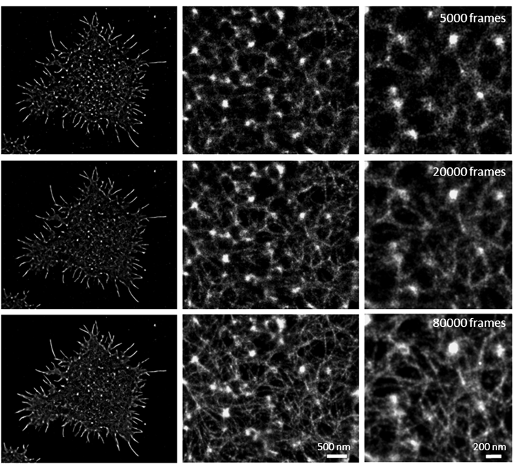
Figure 2. dSTORM images of the actin filaments in primary T cells highlighting the importance of the number of recorded frames necessary to achieve a well defined and continuous actin filament.
Important tips for this section:
- Poor imaging buffer (e.g. not compatible with your fluorophore) will lead to low signal-to-noise ratio, poor localization precision and a low number of localizations resulting in a poor dSTORM image.
- To resolve a structure consisting of your protein of interest you need to record multiple frames. Highly expressed proteins such as actin need thousands of frames with millions of localisations to resolve the fine actin filaments.
Data analysis
After optimizing sample preparation and image acquisition, the final step is to render the single molecule localization datasets. SMLM is a very sensitive method that can detect very small amounts of proteins. However, this comes at a price. Due to its high sensitivity, one needs to be very careful to not introduce artifacts. These can come from several sources such as unclean glass, nonspecific binding of probes, and also from fluorophores that are above or below the imaging focal plane that will be detected and localized. Most of these false positive localizations can be filtered out using the filtering settings during post processing analysis.
Here, we describe the basic filter settings that you can apply to the majority of dSTORM-compatible fluorophores using ONI’s CODI cloud-based platform. Other softwares will likely have similar settings and tools, and the steps should be equivalent.
The first step is to perform drift correction. When recording thousands of frames with blinks from individual fluorophores the image acquisition can take a few minutes and this will lead to drift in your sample. Drift is a consequence of common thermal fluctuations and oil instability within an imaging system. The most commonly used drift correction method is cross-correlation, where the localization dataset is split into individual images created by subsets of frames, which are then correlated to the first image. For example, if 10,000 frames are recorded, these images are split into five individual images each created from 2,000 consecutive frames. These images would then be transformed (shifted) to the first image to correct for drift.
In each frame, the blinks from individual fluorophores are detected, fitted and their coordinates, photon count, localization precision, and other parameters, recorded in the localization list. However, not all the localizations detected meet the basic criteria of acceptance for dSTORM rendering and, therefore, need to be filtered out. The localization precision of the most commonly used fluorophores is usually between 5 and 20 nm. Therefore, using a range of 2-25 nm in CODI will work for most dSTORM-compatible dyes, including fluorescent proteins.
Next, we need to determine what is the width of the Gaussian fit to localize single molecules we want to visualize, i.e. the sigma. As we only want to include molecules that are in the focal plane, a sigma range of 50-250 nm is a good starting point. Additionally, one of the most important parameters is the photon count. This is very important because we only want to visualize molecules with good photon counts, or in other words with high intensity or good signal-to-noise ratio. In CODI you can see the photon count distribution and determine the best value for your fluorophore - usually a value above 300 is a good starting point. After applying these basic filter settings your dSTORM image is now rendered.
The above-mentioned parameters are basic starting settings suggested to minimize the contribution of artifacts associated with imaging. These parameters can be further refined for specific fluorophores. For example, some fluorophores with a good signal-to-noise ratio have histogram distributions of their localisation precisions peaking at around 5 nm. In this case, you should narrow down your localisation precision filter from the recommended range of 2-25 nm to 2-10 nm. The same would apply to other filters.
Important tips for this section:
- Drift correction will not work well if the number of localizations used to render the image in subsequence image subsets is not sufficient to reconstruct your structure of interest.
- You should aim for individual blinking fluorophores with a high signal-to-noise ratio that will translate to a higher photon count and better localization precision.
If you are keen to learn more about the Dos and Don'ts for dSTORM imaging, take a look at Tips & Tricks webinar on The Ins and Outs of mastering dSTORM imaging. For additional queries, including additional hardware settings, other considerations, or if you wish to try the Nanoimager or CODI, visit our website and get in touch with us at hi@team.oni.