The raw data obtained from SMLM experiments, such as dSTORM imaging, is a point cloud of localizations which give us the resolution that we need. However, for the purposes of interpreting our results, we want to relate these localizations to the structures we are interested in. This is where clustering comes in!
We can use different algorithms to cluster localizations together. The resulting clusters, which represent our features of interest, can then be used in further analysis downstream.
How does localization data clustering work?
There are many popular algorithms, but most approaches rely on some metric of density. In general localizations that are densely packed form clusters, and these clusters are separated by areas of sparse localizations. In practice, however, this is a complicated problem. For example, due to the varying background across a sample or because some clusters themselves contain smaller clusters.
On our collaborative discovery platform (CODI) we offer a few different clustering analyses including DBSCAN, HDBSCAN and our own extension of HDBSCAN called Constrained clustering. Behind these methods we use the concept of a cluster tree, which captures different possible clusters by considering how big clusters may break down into smaller clusters.
The cluster tree below represents possible clusters but to get a single cluster result we need to take a ‘cut’ across that tree. Crucially this cut does not allow the same point to be in multiple clusters. For example, we cannot have a result with both the magenta and cyan clusters as they contain some of the same points. In this case some possible results would include:
- One large cluster in white
- Two clusters in magenta and blue
- Three clusters in cyan, purple and blue
- Two clusters in cyan and purple
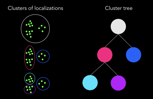
Cluster tree schematic. We can cluster the same green points on the left in different ways. These possible clusters are represented as a hierarchy in the tree on the right. Note that clusters can contain other clusters e.g. the magenta cluster breaks down into the smaller cyan and purple clusters.
What is the difference between these clustering methods?
Here is a brief description to help you best assess which algorithm to choose for your data analysis:
DBSCAN is a commonly used technique and is great for when you have a sample which should form clusters of a uniform density. This algorithm works by building clusters outward from core points, which are localizations that have sufficient nearby neighbors. This algorithm effectively takes a horizontal cut across the cluster tree to select a set of clusters so could yield results like 1, 2 or 4 from the caption above depending on the parameter you set.
DBSCAN has a single parameter which effectively allows you to tune this density. We have made this parameter interactive on our platform so that you can quickly find the best settings for your analysis. Read more about the details of the algorithm in the original DBSCAN paper.
HDBSCAN is another published method, which builds on the density based approach of DBSCAN but also accommodates the hierarchical nature of clusters, i.e. that one cluster may contain smaller clusters. This means it can be useful in samples where we are interested in populations of clusters that may have different densities.
HDBSCAN works by building a tree of all possible clusters, where the root of the tree is one big cluster containing all the points in the dataset. Subsequent branches of the tree are formed as this cluster breaks up into smaller clusters all the way down to a minimum cluster size, as shown in the figure above. The algorithm then looks at each possible cluster and chooses a set of consistent clusters which it considers the most ‘stable’. This will correspond to some cut across the cluster tree which may move up and down in order to select larger or smaller clusters in cases where those are the most stable. This would yield one of the results 1, 2, 3 or 4 from the caption above depending on which was most stable. Read more about the algorithm in the HDBSCAN documentation.
Constrained clustering allows you to cluster according to spatial properties that your cluster should have. This method builds on HDBSCAN by allowing pruning of the cluster tree before selecting the most stable set of clusters. Here pruning means that some nodes on the cluster tree are excluded before using the same HDBSCAN stability metric to select a cut of clusters to include in our results. This pruning can be performed on cluster properties, including skew, area, number of localizations etc. These constraints can also be tweaked in real time. This algorithm was developed at ONI and is available on CODI.
Note that constraints here are not the same as filtering out clusters, which do not meet your criteria. Filtering simply throws out the points from your analysis. Constraining actually allows those points to form different clusters which may be relevant for your analysis. For example, in the image above, HDBSCAN may select the magenta and blue clusters as the most stable cut across the tree. However if you know you expect small round clusters then you could exclude clusters with a high skew (clusters that are long and thin) to eliminate the magenta cluster from the tree. Now the most stable cut across the tree could include those smaller clusters in cyan and purple, which you do want to analyze.
To learn more about these methods and how to practically apply these on the same dataset take a look at our Tips & Tricks webinar on Using Localization Data Effectively.
Applications
Clustering on localization data allows researchers to find biological structures and quantify their morphological properties. This can be applied to a range of biological application, including receptor distribution on T-cells or other cells in the immuno-oncology field, synaptic markers in neuroscience studies, single biomarkers on extracellular vesicles, and nuclear architecture or cell organelles to phenotype diseased or healthy cells, among others.
One example where this can be useful is for studying the molecular mechanisms underlying cancer in patient samples, such as tissue section. For example, dysregulation of multiple biological pathways caused by an increased mutation burden is common in all tumors. These mutations allow cancer cells to evade immune destruction, bypass cell-cycle checkpoints and divide uncontrollably or even change their source of energy by switching to aerobic glycolysis to produce ATP. This shift in the source of ATP results in an altered mitochondrial function which affects mitochondrial morphology.
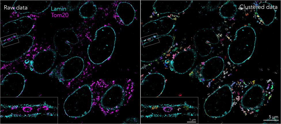
Colorectal cancer tissue sections stained with anti-lamin (cyan) and anti-Tom20 (magenta) to visualize the interior nuclear envelope and mitochondria, respectively (left). Clustering analysis was applied (right) to detect and analyze molecular changes in the diseased tissue.
Super-resolution microscopy in combination with downstream application of clustering algorithms provides an optimal solution to detect the nanoscale changes of mitochondrial morphology which allows researchers and pathologists to monitor the metabolic state of tumors. This improves their ability to stratify patients and find the most suitable therapy or monitor the effect of different therapeutic strategies. It also opens up novel avenues for drug discovery and screening by looking at nanoscale changes in mitochondrial morphology in presence of a therapeutic agent.
Getting started
Using CODI you can perform clustering as part of a seamless analysis workflow. After running the analysis tool you can adjust some parameters interactively and see results update in real time. After you’re happy with your settings you can then go ahead and apply the same exact analysis to different conditions or repeats.
If you’d like to learn more about our CODI platform and try out some clustering yourself then please get in touch!